Bloom Filters

A Memory-Saving Solution for Set Membership Checks

Apr 16, 2025

Hello! Today, we will explore bloom filters—what they are and how they work. Then, we will discuss when and when not to use them before wrapping up with probability insights and key performance considerations. Let’s get started!

Introduction

Imagine we are building a high-traffic service that needs to quickly determine whether a user has visited a page before. Storing every user request in a traditional hashmap would be too memory intensive while querying a database would introduce additional latency.

What if, instead, we could use a data structure that tells us—using just a fraction of memory—whether a user probably visited the page before? This is where bloom filters come in.

A bloom filter is a space-efficient, probabilistic data structure to check for set membership. It returns two possible answers:

The element is definitely not in the set (no false negatives).
The element may be in the set (false positives are possible).

Green shows the results a bloom filter can return; red shows the results it never will:

A bloom filter can return all the options except for false negatives.

At a high level, a bloom filter can be compared to a hashmap, as both rely on hashing. However, they are some key distinctions. Let’s do a quick refresher on hashmaps, then delve into bloom filters to explore their similarities and differences.

Hashmap

A hashmap is a data structure that allows for efficient key-value pair storage and retrieval. There are different implementations, but we will consider a common one based on an array of linked lists.

When a key-value pair is stored in a hashmap, a hash function computes its key and maps it to an index in the array. If multiple keys map to the same index (hash collision), the corresponding linked list stores multiple key-value pairs.

For example, consider the following hashmap:

Suppose we need to store the key-value pair D → qux:

If hashing D gives us index 0, it creates a new linked list at that index.
If hashing D gives us index 1, it appends D → qux to the existing linked list already containing keys A and C.

Hashmaps can also be used for set membership checks. In this case, we only care about the keys, and the values are irrelevant. Some languages, like Java, have a specific data structure called a hashset, which is essentially a hashmap where only the keys are stored.

While hashmaps/hashsets provide efficient storage and retrieval, they can consume significant memory resources as all the elements need to be stored. In contrast, bloom filters allow us to check for set membership with far less memory. Let’s see how that works.

Bloom Filter Introduction

Internally, a bloom filter consists of:

A bitvector (a contiguous sequence of bits).
A fixed size, meaning it can’t be resized over time1.
One or multiple hash functions to distribute elements across the bit vector.

For example, let’s consider a bloom filter of 5 bits. Initially, all bits are set to 0:

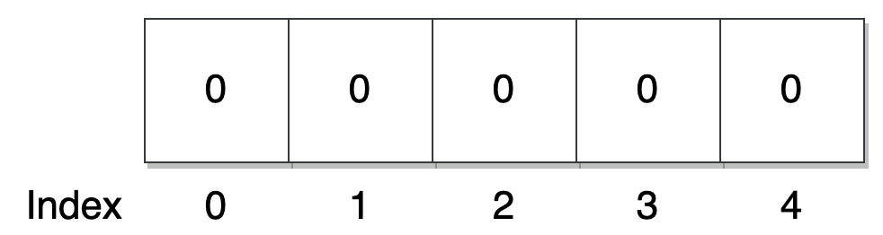
Suppose we want to insert the element “foo“. We will use a hashing function that gives us a value between 0 and 5, say 2, and we set this index to 1:

As you can see, “foo“ isn’t stored in the data structure itself, only its footprint created from the hash function.

Next, we want to insert the element “bar“. We repeat the same operation by calling the same hash function (say it gives us 0 this time) and set the corresponding index to 1:

Now, let’s see how the lookup operation works:

If we want to check if “foo“ is in the bloom filter, we call the same hash function, get index 2, and check the value at this index:
As the value at index 2 is 1, it means the value may be in the set (we will understand the may be part a bit later).
If we want to check if “baz“ is in the bloom filter, we hash the value, and get, for instance, index 4:
Here, as the value of index 4 is 0, the bloom filter can assess that “baz“ is not present in the structure.

Now, let’s cover collisions. So far, we have stored two elements: “foo” and “bar”. Say we want to check whether “qux“ is present in the bloom filter. Unfortunately, hashing “qux“ gives us value 2, which is the same as when we hashed “foo“:

Since index 2 is already set to 1, the bloom filter says that “qux“ may be present.

Indeed, a bloom filter doesn’t know which element was inserted—whether it was “foo“ or “qux“ or some other value. Instead, what it knows is that an element that once hashed to the value 2 was already inserted. This is why a bloom filter returns “may be present“ when a match occurs because of possible hash collisions.

Another important limitation is that we cannot delete an element2. Indeed, if we wanted to reset an index to 0, we wouldn’t know whether this index also corresponds to another element that was already inserted.

In summary, here's a comparison of bloom filters and hashmaps:

Unlike a hashmap, which stores key-value pairs, a bloom filter only stores elements. Furthermore, it doesn’t store these elements explicitly; it only stores their footprints, making it more space-efficient.
A bloom filter is a probabilistic data structure, meaning the results aren’t 100% accurate (as we said, false positives are possible).
We can’t delete data in a bloom filter.

Hashing a Key Multiple Times

Importantly, we should note that bloom filters can be used with multiple distinct hash functions. First, let’s understand how it works and then why we want to do that.

Suppose that instead of using a single hash function, we will use two: MD5 and Murmur. We start with a new bloom filter composed of five elements, and this time, to insert an element, we will call these two hash functions, with each determining one bit position in the bloom filter:

Here, we set both indices 1 and 3 to 1.

Next, we insert “bar“:

Index 1 was already set to 1, so it remains untouched. However, the MD5 function gaves us index 2, so we set it to 1.

This was for the insert operation but the get operation works similarly. Suppose we want to check for the value “baz“:

Here, we need to check all the indices returned by the hashing functions:

If both indices are set to 1, the value may be present in the set.
Otherwise, the value isn’t in the set. Here this is the case here as only index 3 is set to 1.

Therefore, an insert of a lookup has a time complexity of O(k·n) where:

k is the number of hash functions.
n is the length of the element3.

But why are we doing that? Why not use a single hash function? Can you guess?

The reason is to reduce the false positive rate. With k representing the number of hash functions (k = 2 in this example):

A small k increases the false positive rate as only a small number of bits are checked.
A large k reduces the false positive rate but increases the time required for insertion an lookups.

Use Cases

Bloom filters are powerful, but they aren’t always the right tool. Let’s break down when they should not be used and when they shine.

❌ When not to use bloom filters:

When we can tolerate false positives: Bloom filters can tell us that an element might exist, but they can’t guarantee its existence. If a strict guarantee is required, other data structures like hashmaps or B-trees are better.
When deletions are required: Standard bloom filters only support insertions.
When the data set is small: If we’re dealing with a small volume of data, a hashmap is probably more than enough.
When insertions are unbounded: As we discussed, bloom filters have a fixed size. The more elements we add, the higher the false positive rate becomes. This makes bloom filters unsuitable for scenarios where the data set grows indefinitely.

✅ Conversely, the main use case for bloom filters is to act as a memory-efficient way to tell us if an element doesn’t exist in a set. They are widely used in:

Databases: Used to check if a key doesn’t exist, avoiding unnecessary disk lookups. For example, Apache Cassandra uses bloom filters to quickly determine if a row is absent before doing expensive disk reads.
CDNs and caching: Optimizing storage and request efficiency. For example, Akamai’s CDN uses bloom filters to prevent caching webpages that are requested only once.
Blockchain to speed up event searches: Ethereum uses bloom filters to quickly check if a block may contain relevant logs, reducing unnecessary storage and search overhead.
Network security and intrusion detection: Some firewall and DDoS protection systems use bloom filters to efficiently track and filter out bad IP addresses.

Probability

If we know the number of expected elements in the bloom filter, we can use some math to understand how likely false positives are. Let’s define the key parameters:

k: The number of hash functions.
n: The number of expected elements in the bloom filter.
m: The size of the bitvector (in bits).
e: Euler’s number (≈ 2.718)

NOTE: Let’s pause for a second on an important parameter: n. As we discussed, bloom filters have a fixed size and the false positive rate increases with the number of elements added. Making an accurate estimation of n, the number of expected elements, is crucial for the following probabilities as they all depend on this value.

The probability of a false positive when checking for an element is given by:

\(p = \left( 1 - e^{- \frac{k n}{m}} \right)^k\)

For example, if n = 1,000, m = 10 KB, and k = 2, we get a false positive rate of about 3.15%. This formula help us gauge how “reliable“ a given bloom filter configuration is.

NOTE: Some bloom filter libraries provide built-in methods to estimate the false positive rate. For example, Guava’s BloomFilter in Java has the expectedFpp() method to retrieve the expected false positive probability (doc).

Equally interesting: instead of calculating p, we can calculate the value of n, meaning to determine the necessary size of the bloom filter to achieve a specific positive rate. Rearranging the equation:

\(m = -\frac{n k}{\ln(1 - p^{\frac{1}{k}})}\)

For example, if k = 2, n = 1,000, and we want a false positive rate p to be at most 0.1%, we get m ≈ 62,240, which is a bit less that 8 KB.

In my experience, it’s more interesting to approach bloom filters from this angle:

Estimating the expected number of elements (n).
Setting a tolerable false positive rate (p).
Calculating the required bitvector size (m).

Performance

Let’s now discuss performance considerations.

A bloom filter is allocated contiguously in memory, like an array. However, unlike arrays, its access pattern is random due to hash function outputs:

An array traversal (one of the primary access patterns for arrays) is cache-friendly: When the CPU fetches an array’s first element, it pulls in an entire cache line (typically 64 bytes) into the L1 cache. Hence, the subsequent accesses are extremely fast, as they are already in the cache.
Bloom filters suffer from random access: Each bit lookup is determined by a hash function, which may point to different cache lines, leading to multiple memory fetches.

In the worst-case scenario, with k the number of hash functions, checking for an element requires fetching k different cache lines, adding significant latency (if nanoseconds-level performance matters; otherwise, we don’t really care).

Different bloom filter alternatives exist to improve performance. For example, we can mention blocked bloom filters that optimize spatial locality by:

Dividing the bloom filter into small, contiguous blocks, each the size of a cache line.
Restricting each query to a single block ensures all bit lookups stay within the same cache line.

The core idea is to use the first hash function to select which block to access while the remaining functions determine which bits to check within that block.

For example, checking for “foo“ in a two-block structure using k = 3:

A blocked bloom filter internal representation.

The first hash function (hash1) selects the block index; here, 1.
The second and third hash functions (hash2 and hash3) determine the bit positions to be checked within that block (indices 499 and 1538). The rest of the logic remains the same: if both indices are set to 1, the element may be present in the set.

Therefore, in the worst case, instead of accessing two cache lines in this very example, all lookups and inserts remain in one cache line.

Furthermore, a bloom filter shared by multiple threads can introduce false sharing, where different threads modify bits within the same cache line, causing the CPU to frequently synchronize and update cache data between cores, leading to performance degradation.

A more efficient approach could be to rely on blocked bloom filters in a way that:

Each block logically belongs to a single thread, preventing multiple threads from modifying bits within the same cache line.
The first hash function not only determines the block index but also which thread is responsible for handling the lookup or insertion.

This makes blocked bloom filters not only more cache-efficient but also better suited for parallelized workloads.

Summary

A bloom filter is a memory-efficient data structure for set membership checks.
It trades accuracy for space efficiency, allowing false positives but no false negatives.
Ideal for large-scale systems, it helps reduce costly operations like database lookups.
Despite being probabilistic, the false positive rate can be estimated based on factors like the expected number of elements and the number of hash functions.
The standard implementation isn’t cache-friendly. If nanoseconds matter, alternatives like blocked bloom filters should be considered.

💬 Have you ever used bloom filters? Let’s discuss it.

❤️ If you made it this far and enjoyed the post, please consider giving it a like.

📚 Resources

Sources

Explore Further

Bloom filters - Sam Who // Great visualizations.
Modern Bloom Filters: 22x Faster! // If you want to delve into performance considerations.

To be accurate, this limitation applies to the classic bloom filter implementation. However, variants like scalable bloom filters allow dynamic resizing to handle growing data sets, though they come with added complexity and memory overhead.

This limitation also applies to the classic bloom filter implementation. Note that variants like counting bloom filters allow deletions, though they also come with additional complexity and memory overhead.

For variable-length elements, such as strings, hashing complexity scales with the length of the string, meaning it’s not a constant-time operation. Yet, for fixed-size elements, such as a 64-bit integer, hashing runs in O(1) time.